Belief Propagation Converges to Gaussian Distributions in Sparsely-Connected Factor Graphs

We provide the first mathematical proof that local variable beliefs in sparse, spatial AI factor graphs converge to Gaussian distributions via a convolutional CLT mechanism. This theoretical guarantee justifies using efficient Gaussian Belief Propagation over expensive non-parametric methods in non-Gaussian settings.

Abstract

Belief Propagation is a powerful algorithm for distributed inference in probabilistic graphical models, however it quickly becomes infeasible for practical compute and memory budgets. Many efficient, non-parametric forms of BP have been developed, but the most popular is Gaussian Belief Propagation, a variant that assumes all distributions are locally Gaussian. GBP is widely used due to its efficiency and empirically strong performance in applications like computer vision or sensor networks - even when modelling non-Gaussian problems.

In this paper, we seek to provide a theoretical guarantee for when Gaussian approximations are valid in highly non-Gaussian, sparsely-connected factor graphs performing BP (common in spatial AI). We leverage the Central Limit Theorem to prove mathematically that variables' beliefs under BP converge to a Gaussian distribution in complex, loopy factor graphs obeying our 4 key assumptions. We then confirm experimentally that variable beliefs become increasingly Gaussian after just a few BP iterations in a stereo depth estimation task.

Belief Propagation

Belief Propagation (BP) is a distributed probabilistic inference algorithm that computes marginal distributions via iterative message passing on factor graphs.

A factor graph encodes a joint distribution \(p(\mathbf{x}) \propto \prod_s f_s(\mathbf{x}_s)\) as a bipartite graph of variable nodes \(x_i\) and factor nodes \(f_s\). BP passes messages between them with three update rules:

The widget below lets you explore BP on different graph topologies. Each variable has an unknown 2D position; its graph node shows the current belief mean, and the variance ring shows uncertainty (a larger ring means higher uncertainty). The purple diamond marks the true posterior mean for comparison. As messages pass, nodes converge toward the diamond. Click a variable to send messages to its neighbours or send a single random message or run a full synchronous iteration with the buttons below.

For a detailed, interactive introduction to Gaussian Belief Propagation see gaussianbp.github.io, which this was heavily inspired by.

Key Intuitions

We show that Belief Propagation messages converge to a Gaussian distribution in a range of topologies. This is because message passing at factors is equivalent to convolution, and repeated convolution drives distributions to a Gaussian via the Central Limit Theorem. Then at variables, message passing involves multiplying incoming messages, which we show preserves Gaussianity. A surprising range of non-Gaussian problems can then be approximated as Gaussian, and our goal is to encourage the use of GBP over expensive non-parametric methods.

In the demo below, see how factor distributions are messy & noisy, but as you click on variables further from a prior factor, their beliefs become increasingly Gaussian.

Assumptions

Experimental Results

We validate our theoretical findings in stereo depth experiments. In stereo depth estimation, we estimate depth between two stereo images using per-pixel disparity. Disparity is the difference in position between corresponding pixels in the left and right images.

We take a patch around each pixel and compare it to the corresponding patches in the right image, searching across a range from the original position. From this, we build up a probability for each disparity value in the search range.

From these per-pixel disparity distributions, we construct a factor graph that connects each pixel variable to its neighbours, with smoothness factors that encourage nearby pixels to have similar disparities. We run GBP to optimise this non-Gaussian graph because, as our theory predicts, the majority of variable beliefs converge to Gaussian distributions during inference. In general, it is only the highly confident beliefs around textured regions (e.g. edges) that remain non-Gaussian.

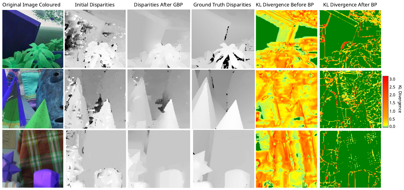
We see that GBP substantially improves disparity estimates over the initial patch-matching baseline across all three scenes. The KL divergence maps then confirm the theoretical prediction: beliefs that are highly non-Gaussian before inference converge to near-Gaussian distributions after BP, particularly in textureless regions where patch-matching leads to high uncertainty.

Limitations & Future Work

There are several limitations to our work. In particular, our guarantees do not directly extend to:

• Non-Euclidean state spaces (e.g. Lie Groups), except where tangent-space approximations are valid
• Factors of degree greater than binary, beyond linear cases of the form \( \phi(\mathbf{x})=g(\mathbf{x}\cdot\mathbf{v}) \) (which reduce to recursive 1D convolutions via auxiliary variables)
• Asynchronous or adaptive message schedules
• Loopy graphs that do not converge to steady state beliefs under synchronous BP
• Graphs where factor distributions are not known

Accordingly, our work opens several useful goals for further research, such as analysis of the speed and stability of cumulant decay under asynchronous BP schedules, or for graphs which do not obey assumptions 3 and 4 (low-degree factors and shift invariance). Moreover, extending our cumulant analysis to uncertainties on Lie Groups presents a critical direction for future work in robust robot perception.

Citation

@inproceedings{yates2026gbpclt,
    title={Belief Propagation Converges to Gaussian Distributions in Sparsely-Connected Factor Graphs},
    author={Yates, Tom and Cheng, Yuzhou and Alzugaray, Ignacio and Akarca, Danyal and Mediano, Pedro A. M. and Davison, Andrew J.},
    booktitle={Proceedings of the 43rd International Conference on Machine Learning (ICML)},
    year={2026}
}